Note
Go to the end to download the full example code.
Tutorial: MagmaForge#
Demonstrates how to use MagmaForge to perform MELTS-style calculations.
Open this code in an executable MyBinder instance (MyBinder links may be slow to load– please be patient!):

Introduction#
MagmaForge is a tool for easily running MELTS-style calculations such as progressive crystallization of liquids. It is designed to be a user-friendly wrapper for the underlying phase model code and equillibration routines available in ThermoEngine. This tutorial demonstrates some of the capabilities available in MagmaForge; it is a work in progress and will be updated over the next few months to demonstrate more capabilities.
Minimum Working Example#
The following code block demonstrates the minimum amount of code necessary to run an equilibrium crystallization routine using MagmaForge. In the following sections, we will go through each part and demonstrate additional capabilities.
from thermoengine import magmaforge
import pandas as pd # a useful data analysis package

morb_oxides = pd.Series({
            'SiO2':  48.68,
            'TiO2':   1.01,
            'Al2O3': 17.64,
            'Fe2O3':  0.89,
            'Cr2O3':  0.0425,
            'FeO':    7.59,
            'MgO':    9.10,
            'CaO':   12.45,
            'Na2O':   2.65,
            'K2O':    0.03,
            'P2O5':   0.08,
            'H2O':    0.2},) # Values in grams (extensive units)

sys = magmaforge.System(comp = morb_oxides,
                        P_bar = 1000.0, # bars
                        T_C = 1300, # C
                        logfO2 = ('QFM',-1), # setting fO2 equal to 1 log unit below the QFM buffer
                        database='MELTS_v1_0', # liquid model name
                        )

sys.crystallize(
      method='equil', # equilibrium crystallization
      T_step=10, # decrease in temperature at each step
      fix_fO2=True, # hold fO2 constant at initial fO2 value, relative to indicated buffer
              )

magmaforge.plot.phase_fractions(sys.history)

/workspaces/ThermoEngineLite/thermoengine/thermoengine/magmaforge/system.py:251: UserWarning: Warning: Setting an fO2 value will redistribute the FeO and Fe2O3 values given.
  warnings.warn('Warning: Setting an fO2 value will redistribute the FeO and Fe2O3 values given.')
Breaking It Down#
1. Initialization#
To use MagmaForge, you’ll first need to import the ThermoEngine package and the MagmaForge module. If you’re running the code locally, you should have already installed ThermoEngine to your computer– here you’re importing it from your computer’s package library into this notebook. If you’re running the code via MyBinder, ThermoEngine is already installed by default in the virtual environment.
from thermoengine import magmaforge
Import Pandas (https://pandas.pydata.org/), a package which provides convenient capabilities for entering, storing, and anaylzing data. If you used Anaconda to create a virtual environment on your machine, Pandas should exist on your machine and the import statement below should work. If you get an error message, you can install Pandas by typing “pip install pandas” into your command line.
import pandas as pd
2. Defining a System#
The first step for most MELTS-style calculations is to define a chemical system– i.e., a bulk chemical composition equilibrated at a set of conditions (usually pressure and temperature, but sometimes other variables like entropy or volume). Here, let’s imagine that we’re interested in a mid-ocean ridge basalt. We can define the bulk chemical composition using a series, which is a data type specific to the Pandas package– the ‘pd’ indicates that we are invoking this package.
morb_oxides = pd.Series({
            'SiO2':  48.68,
            'TiO2':   1.01,
            'Al2O3': 17.64,
            'Fe2O3':  0.89,
            'Cr2O3':  0.0425,
            'FeO':    7.59,
            'MgO':    9.10,
            'CaO':   12.45,
            'Na2O':   2.65,
            'K2O':    0.03,
            'P2O5':   0.08,
            'H2O':    0.2},) # values in grams (extensive units)
Now that we have a bulk chemical composition, we can use MagmaForge to equilibrate the MORB composition at the conditions of interest. We use the magmaforge.System() call to create a system object at the indicated composition, pressure, temperature, and fO2. Here, the initial temperature is chosen to be above the liquidus of the system so that later calculations can crystallize the system.
sys = magmaforge.System(comp = morb_oxides,
                        P_bar = 1000.0, # bars, but kbar and GPa may be given as well (see below)
                        T_liquidus = True, # system will equilibrate just above the liquidus; T_C or T_K may be given instead (see below)
                        logfO2 = ('QFM', -1), # setting fO2 equal to 1 log unit below the QFM buffer
                        database='MELTS_v1_0', # liquid model name-- MELTS_v1_0 and MELTS_v1_2 are the most commonly used
                        )
/workspaces/ThermoEngineLite/thermoengine/thermoengine/magmaforge/system.py:251: UserWarning: Warning: Setting an fO2 value will redistribute the FeO and Fe2O3 values given.
  warnings.warn('Warning: Setting an fO2 value will redistribute the FeO and Fe2O3 values given.')
Composition input options: Bulk composition may be input as either a Pandas Series (as shown above) or as a standard Python dictionary. Compositions are currently expected to formatted as weight oxides. If your composition is in another form (e.g. moles of elements), you can use the RockyChem module to convert to weight oxides. Oxides that are not included in the database will be ignored.
Temperature input options: Valid temperature input arguments are ‘T_C’, ‘T_K’, or ‘T_liquidus’. T_C and T_K should be set to numerical values, while T_liquidus=True will equilibrate the system just above the liquidus.
Pressure input options: Valid pressure input arguments are ‘P_bar’, ‘P_kbar’, or ‘P_GPa’.
Redox input options: Redox may be set in one of four ways:
logfO2: as shown above, logfO2 may be set using a tuple of a buffer and an offset, e.g. logfO2=(‘NNO’,-1). If set, the system will redistribute Fe between FeO and Fe2O3 to reach the desired logfO2.
Fe3_tFe: the bulk molar Fe3+/(Fe3+ + Fe2+) ratio at which to equilibrate the system. If set, the system will redistribute Fe between FeO and Fe2O3 to reach the desired ratio.
bulk_Fe2O3: the bulk system Fe2O3 (in wt%) at which to equilibrate the system. If set, the system will redistribute Fe between FeO and Fe2O3 to reach the desired bulk Fe2O3 (per 100 wt% oxides). If the initial composition already contains Fe2O3, this Fe2O3 content will be re-assigned as FeO and then redistributed to thebulk Fe2O3 value provided.
Database input options: Valid databases are:
‘MELTS_v1_0’ (rhyoliteMELTS)
‘MELTS_v1_2’ (rhyoliteMELTS + H2O-CO2 fluid)
‘MELTS_pMELTS’ (pMELTS)
More info: https://melts.ofm-research.org/Support/Understanding-rhyolite-MELTS-versions.html
Further details for System arguments can be found in the API: https://thermoenginelite.readthedocs.io/en/magmaforge_ui/api/magmaforge_system.html#thermoengine.magmaforge.system.System
The sys object that we created in the last cell represents our equilibrated chemical system. We can probe this system to ensure our calculation had the expected behavior. For instance, in the cell below, we are querying the temperature (in K), pressure (in bars), and melt fraction of the system.
print('T (°C): ', sys.T_C)
print('P (bar)', sys.P_bar)
print('F: ', sys.melt_fraction)
T (°C):  1229.9363793483471
P (bar) 1000.0
F:  1.0
3. Performing a Calculation Along a Path#
Now that we have our chemical system, we can perform calculations such as crystallization during cooling. To do this, we will apply the crystallize method to our system. We tell it that we want to use the ‘equil’ (equilibrium/batch crystallization) method of crystallizing, that we want to decrease in temperature steps of 15°, and that we want to hold fO2 steady at the value we set for the system– here QFM -1.
sys.crystallize(
      method='equil', # equilibrium crystallization
      T_step=10, # decrease in temperature at each step, in K
      fix_fO2=True, # hold fO2 constant at the initial relative fO2 value (i.e, here fO2 is held constant at QFM -1)
              )
<thermoengine.magmaforge.system.System object at 0xffffa4d29b10>
Crystallize() input arguments:
method: ‘equil’ for batch/equilibrium crystallization, ‘frac’ for fractional crystallization
fix_fO2: ‘True’ to run buffered at the current logfO2, relative to buffer given during system initialization (open system); ‘False’ to run unbuffered (closed system)
T_step: The temperature interval to adjust T at each step. Both positive and negative values will move system to lower temperature. By default 15.
melt_frac_cutoff: The melt fraction cutoff for declaring crystallization complete, by default 0.01 (1% melt remaining).
T_final_K or T_final_C: The final temperature for the system, if full crystallization is not reached first.
frac_remains: The amount of melt retained at each step during fractional melting, by default 1e-2.
Accessing/Plotting Output#
1. Accessing Output as a Plot#
Once you have performed your calculations, you probably want to see the results. MagmaForge has a few built-in plotting functions for creating basic plots. MagmaForge has a few simple built-in plots that can be called using the magmaforge.plot submodule. Here we’re using the .phase_fractions() method to create an automatic plot of phase fractions with respect to temperature as the system cools. The sys.history object contains the history of the system’s state after each calculation and will be very useful for accessing output.
magmaforge.plot.phase_fractions(sys.history)

For a somewhat more in-depth look at our results, we can use magmaforge.plot.magma_evolution() to plot the phase fractions and magma composition during crystallization.
magmaforge.plot.magma_evolution(sys.history)

You can, of course, also create custom plots using the output of the run. We’ll show some examples of how to access more properties in a later section.
2. Accessing Output as a Table#
You may also want to access numerical output for your run. Recall that the sys.history object stores the information of the state of the system after each calculation. We can access a table showing the fractions of each phase after each calculation step using the .get_phase_frac_table() method. Here we’re using the ‘present’ argument to only display columns for phases that are present at some point during the run.
#Uncomment the row below to see all table rows
#pd.set_option('display.max_rows', None)

sys.history.get_phase_frac_table(phases='present', index='T_C')
The composition of the liquid can be accessed using the .get_phase_comp_table() method:
sys.history.get_phase_comp_table('Liquid', index='T_C')
The composition of phases can also be accessed using the .get_phase_comp_table() method:
sys.history.get_phase_comp_table('Feldspar', index='T_C')
Any of these tables can be easily downloaded as a csv file using built-in Pandas commands, or a table of full results can be downloaded using MagmaForge:
If you are running in a MyBinder, be sure to download your output file to your machine before closing your session!
table_to_export = sys.history.get_phase_frac_table(phases='present')
table_to_export.to_csv('output.csv', index=True)

sys.history.save_full_state_history_table(filename='full_output.csv', P_unit='bar', T_unit='C', fO2_buffer='QFM')
3. Accessing Outputs as Variables/Data Structures#
You can also access each property of the system history as an array or other data structure, which can be helpful if you want to do further math with the outputs. The code below demonstrates many of the methods and properties that can be called. Full documentation of methods and functions can be found in the MagmaForge API reference: https://thermoenginelite.readthedocs.io/en/latest/api/index.html
# System Conditions
T = sys.history.get_temperatures('C')
P = sys.history.get_pressures('bar')
S = sys.history.get_total_entropies()
logfO2 = sys.history.get_logfO2s('QFM')
mass_tot = sys.history.get_total_masses()
bulk_comp = sys.history.get_bulk_comps('wt_oxides') # can also choose wt_elems, mol_elems, or mol_oxides

# Phase Masses
F = sys.history.get_melt_fractions('instantaneous') # can choose 'aggregated', if running fractional
phase_masses = sys.history.get_all_phase_masses()
phase_fracs = sys.history.get_all_phase_fractions()
phase_frac_table = sys.history.get_phase_frac_table(index='T_C')

# Phase Compositions
liq_comp = sys.history.get_phase_comps('Liquid') # can optionally provide unit, by default unit='wt_oxides'
phase_comp = sys.history.get_phase_comps('Feldspar', unit='mol_elems')
phase_comp_table = sys.history.get_phase_comp_table('Feldspar', index='T_C')
liquid_SiO2 = sys.history.get_phase_comp_table('Liquid')['SiO2']

# Other Properties
S_liq = sys.history.get_phase_entropies('Liquid')
V_liq = sys.history.get_phase_volumes('Liquid')
rho_liq = sys.history.get_phase_densities('Liquid')

# Fractional Crystallization/Melting
# frac_mass = sys.history.get_fractionated_masses() # if running fractional
# frac_comp = sys.history.get_fractionated_comps() # if running fractional

print(T) # replace with whichever variable you'd like to view
[1229.93637935 1219.93637935 1209.93637935 1199.93637935 1189.93637935
 1179.93637935 1169.93637935 1159.93637935 1149.93637935 1139.93637935
 1129.93637935 1119.93637935 1109.93637935 1099.93637935 1089.93637935
 1079.93637935 1069.93637935 1059.93637935 1049.93637935 1039.93637935
 1029.93637935 1019.93637935 1009.93637935  999.93637935  989.93637935
  979.93637935  969.93637935  959.93637935]
4. Creating Custom Plots#
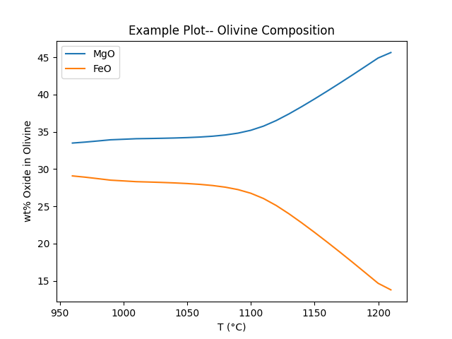
You can also use Matplotlib’s PyPlot module to create custom plots. PyPlot is well-documented and easy to use (tutorial here: https://matplotlib.org/stable/tutorials/pyplot.html). An example is shown below.
import matplotlib.pyplot as plt

# Get data
T_C = sys.history.get_temperatures('C')
MgO_olv = sys.history.get_phase_comp_table('Olivine')['MgO']
FeO_olv = sys.history.get_phase_comp_table('Olivine')['FeO']

# Plot data
plt.plot(T_C, MgO_olv, label='MgO')
plt.plot(T_C, FeO_olv, label='FeO')

# Format plot and axes
plt.title('Example Plot-- Olivine Composition')
plt.xlabel('T (°C)')
plt.ylabel('wt% Oxide in Olivine')
plt.legend()

# Display plot
plt.show()
5. Next steps#
Hopefuly this tutorial gave you a sense of how to use MagmaForge to run MELTS-like calculations.
For more examples of specific functionality, such as fractional melting or isentropic decompression melting, see the MagmaForge section in the Gallery: https://thermoenginelite.readthedocs.io/en/magmaforge_ui/auto_examples/index.html
For a complete documentation of methods and functions, see the MagmaForge API reference: https://thermoenginelite.readthedocs.io/en/latest/api/index.html
Total running time of the script: (0 minutes 24.851 seconds)