Rhyolite-MELTS Geobarometer for silicic rocks

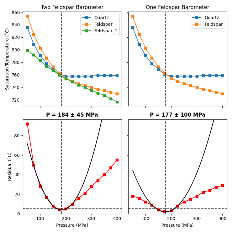
Implements the rhyolite-MELTS geobarometer described by Gualda & Ghiorso (2014) based on the co-saturation of quartz and one or two feldspars. See the manuscript for more information.

Open this code in an executable MyBinder instance (MyBinder links may be slow to load– please be patient!):

Initialization

Import necessary packages:

from thermoengine import magmaforge, model
import numpy as np
from numpy.polynomial import Polynomial
import pandas as pd
import matplotlib.pyplot as plt

Input the bulk rock composition:

# Early Bishop Tuff B7-1 (Anderson et al., 2000)
rhyolite_wtpt = pd.Series({
    'SiO2': 77.6,
    'Al2O3': 12.6,
    'FeO': 0.67,
    'MgO': 0.02,
    'CaO': 0.44,
    'Na2O': 4.15,
    'K2O': 4.67,
    'H2O': 10.0 # Set to a value to ensure fluid saturation
})

# Quartz hosted glass from late-erupted Bishop Tuff (Anderson et al., 2000)
# rhyolite_wtpt = pd.Series({
#     'SiO2': 77.6,
#     'Al2O3': 12.2,
#     'Na2O': 3.54,
#     'K2O': 5.5,
#     'CaO': 0.47,
#     'FeO': 0.69,
#     'MgO': 0.03,
#     'H2O': 10.0 # Set to a value to ensure fluid saturation
# })

Set calculation parameters (or use defaults):

P_min = 50 # MPa
P_max = 400 # MPa
n_P = 15 # Number of pressures to run
dT = 1 # K, the T steps during cooling
Delta_QFM = 0.0

Suppress other phases to increase calculation speed:

db = model.Database('MELTS_v1_0')
phases_to_keep = ['Fsp', 'Liq', 'Qz', 'H2O']
all_phases = db.phase_list
phases_to_remove = []
for ph in all_phases:
    if ph not in phases_to_keep:
        phases_to_remove.append(ph)
db.remove_phases(phases_to_remove)
db.activate()

Run the calculations

This will take a while. To speed things up (but get worse results) decrease the T step above, or the number of pressure steps.

P_to_run = np.linspace(P_min, P_max, n_P)
phase_fracs = []
kfsp_id = np.zeros(n_P)

for i in range(n_P):
    print(f"Starting Calculation {i+1} of {n_P}...")
    sys = magmaforge.System(comp=rhyolite_wtpt,
                            T_C=900.0,
                            P_GPa = P_to_run[i]/1000.0,
                            logfO2 = ('QFM', Delta_QFM),
                            database=db,
                            )

    sys.crystallize(method='equil',
                    T_final_C=700,
                    T_step=dT,
                    fix_fO2=True,
                    )

    phase_fracs.append(sys.history.get_phase_frac_table())

Starting Calculation 1 of 15...
Starting Calculation 2 of 15...
Starting Calculation 3 of 15...
Starting Calculation 4 of 15...
Starting Calculation 5 of 15...
Starting Calculation 6 of 15...
Starting Calculation 7 of 15...
Starting Calculation 8 of 15...
Starting Calculation 9 of 15...
Starting Calculation 10 of 15...
Starting Calculation 11 of 15...
Starting Calculation 12 of 15...
Starting Calculation 13 of 15...
Starting Calculation 14 of 15...
Starting Calculation 15 of 15...

Process Calculation Results

This cell must be run following the calculations, but you can ignore its contents

phase_in = np.zeros([n_P, 3])
residuals = np.zeros([n_P])
residuals_1f = np.zeros([n_P])
phase_names = ['Quartz', 'Feldspar', 'Feldspar_1']
for i in range(n_P):
    table = phase_fracs[i]
    for j in range(len(phase_names)):
        ph = phase_names[j]
        if ph in table:
            phase_in[i,j] = table[table[ph]>0].index[0]
        else:
            phase_in[i,j] = np.nan
    residuals[i] = np.sum(np.abs(phase_in[i,:] - np.nanmin(phase_in[i,:])))
    residuals_1f[i] = np.abs(phase_in[i,0] - phase_in[i,1])

def get_poly_fit(residuals):
    min_point = np.nanargmin(residuals)
    fit_start = np.max([0, min_point - 2])
    fit_end = np.min([n_P, min_point + 3])
    fit = Polynomial.fit(P_to_run[fit_start:fit_end], residuals[fit_start:fit_end], deg=2)
    x, y = fit.linspace(100, (P_min, P_max))
    return x, y

x, y = get_poly_fit(residuals)
x1f, y1f = get_poly_fit(residuals_1f)

Produce a plot of the results

This recreates a plot similar to those used by Gualda & Ghiorso (2014), see the paper for information on how to interpret them.

fig, ax = plt.subplots(2,2, figsize=(7.4,7.4), sharex='col', sharey='row')

for j in range(len(phase_names)):
    ax[0,0].plot(P_to_run, phase_in[:,j] - 273.15, marker='s', label=phase_names[j])
for j in [0,1]:
    ax[0,1].plot(P_to_run, phase_in[:,j] - 273.15, marker='s', label=phase_names[j])

ax[1,0].plot(P_to_run, residuals, marker='s', c='r')
ax[1,1].plot(P_to_run, residuals_1f, marker='s', c='r')
ax[1,0].set_ylim(0, ax[1,0].get_ylim()[1])
ax[1,0].plot(x, y, c='k')
ax[1,1].plot(x1f,y1f, c='k')

ax[0,0].set_title('Two Feldspar Barometer')
ax[0,1].set_title('One Feldspar Barometer')
if np.min(y) < 5.0:
    ax[1,0].set_title(f"P = {x[np.argmin(y)]:.0f} ± 45 MPa", fontweight='bold')
    ax[0,0].axvline(x[np.argmin(y)], c='k', ls='--')
    ax[1,0].axvline(x[np.argmin(y)], c='k', ls='--')
else:
    ax[1,0].set_title("No fit.", fontweight='bold')
if np.min(y1f) < 5.0:
    ax[1,1].set_title(f"P = {x1f[np.argmin(y1f)]:.0f} ± 100 MPa", fontweight='bold')
    ax[0,1].axvline(x1f[np.argmin(y1f)], c='k', ls='--')
    ax[1,1].axvline(x1f[np.argmin(y1f)], c='k', ls='--')
else:
    ax[1,1].set_title("No fit.", fontweight='bold')

ax[1,0].axhline(5, c='k', ls='--')
ax[1,1].axhline(5, c='k', ls='--')

ax[0,0].legend()
ax[0,1].legend()

ax[1,0].set_ylabel('Residual (˚C)')
ax[0,0].set_ylabel('Saturation Temperature (˚C)')
ax[1,0].set_xlabel('Pressure (MPa)')
ax[1,1].set_xlabel('Pressure (MPa)')

fig.tight_layout()

plt.show()